Published 19 June 2014 by Wolfgang Huang
Latex Support
We have been asked to include LaTeX support for our blog. And here it is!
You may also use display environments equation, align, displaymath, eqnarray, multline, flalign, gather, and alignat.
Here is an example:
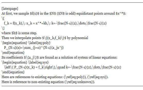
The above code is rendered as:
At first, we sample $f(x)$ in the $N$ ($N$ is odd) equidistant points around $x^*$:
[
f_k = f(x_k),: x_k = x^*+kh,: k=-frac{N-1}{2},dots,frac{N-1}{2}
]
where $h$ is some step.
Then we interpolate points ${(x_k,f_k)}$ by polynomial
begin{equation} label{eq:poly}
P_{N-1}(x)=sum_{j=0}^{N-1}{a_jx^j}
end{equation}
Its coefficients ${a_j}$ are found as a solution of system of linear equations:
begin{equation} label{eq:sys}
left{ P_{N-1}(x_k) = f_kright},quad k=-frac{N-1}{2},dots,frac{N-1}{2}
end{equation}
Here are references to existing equations: (ref{eq:poly}), (ref{eq:sys}).
Here is reference to non-existing equation (ref{eq:unknown}).
For the display environments, equation numbering is automatic, but this may be overridden and the number set explicitly with tag{..} placed within the display expression.
A number of options may be set for an expression with attribute tags such as size, color, background, align, as arguments of quicklatex{} placed within the expression:
renders with green font of 25 pixels height:

Compilation of an expression may be suppressed, showing instead the LaTeX source, by preceding the expression with a !.
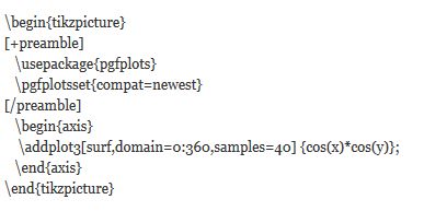
For mathematical graphs you may use tikzpicture and pgfplots, e.g. :
compiles to

Realized with WP QuickLaTeX.


